Ranjeet Gupta
Portfolio / Overview

M.TECH · GEOSPATIAL ENGINEERING · IIT ROORKEE

Turning Earth observations into decisions.

I am Ranjeet Gupta, a geospatial engineer working across GeoAI, remote sensing, computer vision, spatial data engineering and operational AI. This portfolio explains what I built, how it works, what the evidence shows and where the limitations remain.

Portrait of Ranjeet Gupta
GeoAI · Remote sensing · Computer vision
AIR 153 GATE 2025
94th WorldQuant global
0.9369 Antariksh mAP@10
0.706 Building IoU

My research map

Reliable geospatial products connect four layers instead of optimizing a model in isolation.

Observe Optical · SAR · LiDAR
→
Model GeoAI · CV · statistics
→
Operate MLOps · drift · telemetry
→
Decide Maps · explanations · action

Featured work

PROFILE

From pixels to operational products.

My foundation combines remote sensing and GIS with machine learning, image processing, databases and software development.

Education

M.Tech, Geospatial Engineering · IIT Roorkee

CGPA 7.718. Earth observation, GeoAI, photogrammetry and operational geospatial systems.

M.Tech coursework, Geoinformatics · IIST (ISRO) Thiruvananthapuram

Completed two semesters before discontinuing the programme (CGPA 7.14). Coursework included remote sensing, GIS, scientific computing, digital photogrammetry and UAV remote sensing, geospatial modelling, machine learning, computer vision and active remote sensing.

B.Tech, Geoinformatics · NSUT Delhi

CGPA 8.23. GIS, remote sensing, GNSS, spatial databases and programming.

Academic transition: the IIST programme was discontinued after two completed semesters; the foundation built there now supports the ongoing M.Tech work at IIT Roorkee.

Location & professional links

HOME BASEMumbaiPersonal home location
WORK PREFERENCEDelhi → BangaloreFirst preference Delhi; second preference Bangalore
LINKEDINranjeetgupta-nsutOpen profile ↗

Working principles

Understand the sensor

Verify resolution, spectral meaning, CRS and NoData before modelling.

Build an auditable method

Give every transformation a reason and measurable output.

Separate evidence from assumption

Report candidates and limitations honestly.

Deliver for decisions

Translate analysis into maps, vectors, interfaces or alerts.

M.TECH THESIS · IIT ROORKEE · JUL 2026–PRESENT

InundraONE: flood intelligence as an operational GeoAI system

An AOI-driven WebGIS that turns Sentinel-1 SAR scenes into flood extent, depth and exposure evidence—then publishes every event as a traceable, decision-ready map.

What the thesis is building

Flood mapping is not finished when a model produces a raster. A useful system must find the right acquisition, preserve event lineage, remove persistent water, estimate defensible depth, intersect exposure layers and serve the result fast enough for exploration. InundraONE connects that full chain for Lakhimpur.

Research question How can one operational pipeline convert a selected Sentinel-1 event into reproducible flood-risk evidence while retaining the observability, auditability and safeguards expected from AIOps?
Single-SAR event-wise flood detection
4 classes land · flood · water · NoData
80% persistent-water threshold
AOI + event storage and provenance key
AOI user-defined boundary
→
Acquire Sentinel-1 GRD
→
Prepare VV dB · clip · mosaic
→
Segment Otsu + Chan–Vese
→
Refine majority + permanent water
→
Depth FABDEM + FwDET
→
Expose crop · building · road
→
Publish COG · API · WebGIS

Detection logic, step by step

01 · Scene selection and event integrity

An event uses one Sentinel-1 acquisition context. Adjacent GRD slices may be mosaicked only when acquisition date, relative orbit and pass direction match; this prevents unrelated radar geometries from being treated as one observation.

02 · Backscatter thresholding

VV intensity is converted to decibels and clipped to the AOI. Otsu selects the threshold that maximises between-class variance, providing a data-driven initial separation of dark water-like returns from land.

03 · Spatial refinement

Morphological Chan–Vese regularises the thresholded region by balancing region statistics with boundary smoothness. A 3×3 majority filter then suppresses isolated speckle without pretending that radar intensity alone proves flooding.

04 · Permanent-water separation

Dynamic World observations from the preceding 365 days estimate water persistence. Pixels classified as water in at least 80% of a minimum three observations are labelled permanent water, not event flood.

05 · Depth and exposure

FwDET propagates the nearest flood-boundary elevation through the inundated region. Depth is then sampled against crop parcels, Google Open Buildings footprints (confidence ≥0.7) and buffered OpenStreetMap roads to convert extent into consequences.

The mathematics behind the map

t* = arg maxt σ²B(t)

Otsu threshold. Choose the split whose two intensity groups are most separated. This initializes water-like pixels without a hand-picked global constant.

Pwater(x) = (1/N) Σ 1[labeli(x)=water]

Persistence. If Pwater(x) ≥ 0.80 with N ≥ 3, the pixel becomes permanent water and is excluded from the flood-only class.

d(x) = max(0, DEM(b*(x)) − DEM(x))

FwDET depth. b*(x) is the nearest flood-boundary pixel. Its terrain elevation approximates water-surface elevation; negative depths are clipped to zero.

BUILDINGSlow 0–0.5 mmoderate 0.5–1.5 m · high >1.5 m
ROADSlow 0–0.3 mmoderate 0.3–1.0 m · high >1.0 m
OUTPUT MASK0 · 1 · 2 · 255land · flood · permanent water · outside/NoData

System architecture and AIOps boundary

DATASentinel-1 · FABDEM · Dynamic World · OSM · Open BuildingsVersioned inputs tied to AOI and event identity
↓
PROCESSINGPython geospatial pipelineSearch · COG preprocessing · mask · depth · exposure · statistics
↓
SERVICESFastAPI + TiTilerCOG, GeoJSON and JSON outputs exposed as map and analytics endpoints
↓
EXPERIENCENext.js + React + MapLibreAOI history, event selector, layers, legends and impact summaries

Current scope: the event-processing and interactive WebGIS design are established. Field/gauge validation, population-village-shelter layers, scheduled orchestration and full AWS AIOps deployment remain planned work—not completed claims.

Seminar walkthrough

Watch the complete presentation to see the literature gaps, proposed architecture and responsible deployment controls explained as one connected system.

17:41 · SEMINAR

Geospatial AIOps in Earth Observation

Critical review and a unified operational framework for scalable, observable, adaptive and trustworthy EO systems.

WORLDQUANT BRAIN · 2023–2025

Quant research as a disciplined experiment.

I researched predictive financial models across 34,000+ fields, tested them on defined universes and refined their balance of performance, risk and trading activity. Proprietary signals are not disclosed.

Research lifecycle

Hypothesis Economic rationale
→
Data Relevant fields
→
Expression Valid operators
→
Simulate Returns + risk
→
Stress-test Robustness
→
Document Rationale + lineage

Evaluation framework

Sharpe ≈ mean(returns) / std(returns)

Risk-adjusted consistency; it still needs stability checks.

Turnover = traded value / portfolio value

High activity can make an attractive model inefficient.

Fitness = performance × efficiency

Balances predictive strength instead of optimizing one metric.

Result: 94th global rank in the 2025 PowerPool Alpha Competition. LLM-assisted exploration can translate hypotheses into valid candidate expressions, but compilation, simulation and robustness—not generation—remain the evidence gate.

VERIFIED COMPETITIVE MILESTONES

From an institute Alphathon to the global PowerPool field.

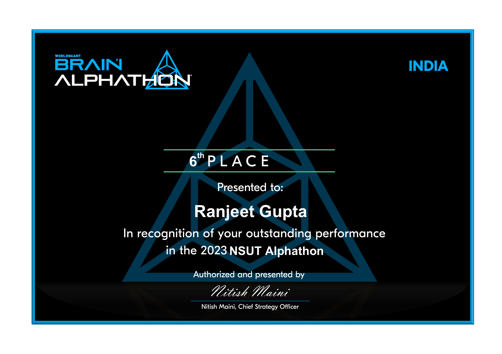
The two certificates show progression across distinct competitions. The 2023 result records 6th place in the NSUT Alphathon; the 2025 PowerPool certificate records 94th globally and 26th in India. They support the result claims without exposing proprietary alpha expressions.

2023 NSUT Alphathon · 6th place 2025 PowerPool · 94th global · 26th India
WorldQuant PowerPool Alpha Competition 2025 certificate showing Ranjeet Gupta ranked 94th globally and 26th in India
PowerPool Alpha Competition 2025 · 94th global · 26th in India.
WorldQuant Brain certificate awarding Ranjeet Gupta sixth place in the 2023 NSUT Alphathon
WorldQuant Brain NSUT Alphathon 2023 · 6th place.

HIWARA ENGINEERS · 2026

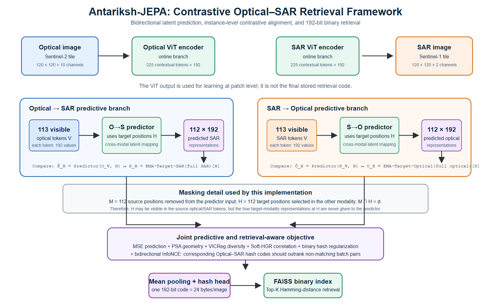
Antariksh-JEPA: Optical ↔ SAR retrieval

A bidirectional system that learns shared meaning between Sentinel-2 optical and Sentinel-1 SAR tiles, then retrieves compact 192-bit codes with Hamming distance.

0.9036 Optical→SAR mAP@10
0.9369 SAR→Optical mAP@10
24 bytes per image code

Why it matters

Optical data is intuitive but cloud-limited; SAR observes structure through cloud and darkness. Cross-modal retrieval lets an analyst query one and inspect semantically related observations in the other.

Antariksh-JEPA architecture
Dual ViT encoders, masked bidirectional latent prediction, retrieval-aware alignment, binary hashing and FAISS search.
Pair BigEarthNet-MM
→
Encode Optical/SAR ViTs
→
Align Predictive + contrastive
→
Hash 192 bits
→
Retrieve Hamming top-k

IIST · 2025

Automated building-footprint extraction

An instance-segmentation pipeline trained on labelled US aerial imagery and evaluated on an Indian test area, producing map-ready polygons.

0.706 validation IoU
966 polygons
0.784 mean confidence

Architecture and training

512² RGB Tiles + masks
→
ResNet-50 FPN Multi-scale features
→
RPN Candidate regions
→
RoIAlign Aligned features
→
Heads Class · box · mask

Overture polygons became instance masks. A COCO-pretrained Mask R-CNN was fine-tuned for 100 epochs in recorded experiments. Joint loss combines classification, box, mask and proposal losses.

Mask → GIS polygon

  1. Overlapping 512×512 inference windows reduce edge loss.
  2. Confidence filtering removes weak detections.
  3. NMS compares overlap by IoU and keeps the strongest duplicate.
  4. Mask boundaries become georeferenced polygons.
  5. Simplification and attribute filters regularise geometry.

Limitation: small, dense, irregular and shadowed buildings remain difficult. Kochi generalisation is evidence of transfer, not universal accuracy.

Project walkthrough

PROJECT VIDEO

Mask R-CNN for map-ready building polygons

A narrated view of the problem, training pipeline, inference and GIS output.

IIT ROORKEE · SCIENTIFIC COMPUTING · 2023 DELHI FLOOD

Sentinel-1 flood monitoring—evidence from backscatter change.

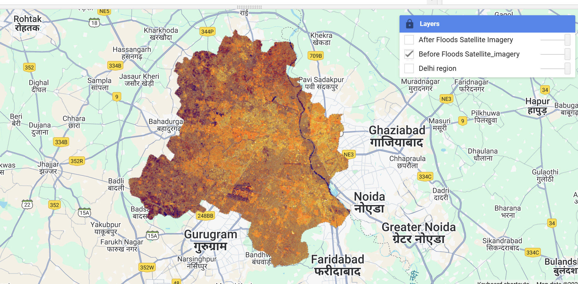
A Google Earth Engine workflow compares pre- and post-event Sentinel-1 VV/VH mosaics, suppresses speckle, detects a water-like backscatter drop and removes known false positives before estimating inundated area.

21,717.53 ha mapped flood extent
14.6% derived share of ROI
10 m input SAR resolution
1.25 implemented ratio threshold

From radar signal to a defensible flood mask

Acquire Sentinel-1 IW · VV/VH
→
Mosaic pre / post windows
→
Filter Refined Lee
→
Detect change threshold
→
Clean water · slope · connectivity
→
Measure pixel-area sum
Ilin = 10IdB/10

Refined Lee filtering is applied in natural-intensity space, then converted back using IdB = 10 log10(Ilin). Directional local statistics reduce multiplicative speckle while retaining edges.

M = 1[C > 1.25] · 1[Wperm=0] · 1[slope<5°] · 1[Nconn>8]

The submitted code uses C = postdB/predB . Because dB values are negative, the ratio convention and the report’s Δσ⁰ < −1.25 dB wording are not interchangeable; a production version should select one calibrated convention explicitly.

Aflood = Σp M(p)·A(p)

GEE sums the area of retained pixels. The logged values yield 21,717.53 / 148,752.77 × 100 = 14.6%. The presentation labels this “20%”; the portfolio reports the arithmetic result and flags the mismatch.

DATES & FILTERS

What the model sees

Pre-flood imagery spans 15 June–3 July 2023; post-flood imagery spans 3–21 July 2023. Permanent or seasonal water is removed with JRC Global Surface Water seasonality ≥5 months, slope is constrained with HydroSHEDS, and isolated components are filtered.

5° slope cutoff in code 8 px connectivity cutoff 30 m area-reduction scale

Interpretation: smooth open water generally returns less energy to the sensor, but urban double-bounce, vegetation and incidence geometry can violate that assumption. This is a change-detection product—not direct water-depth measurement.

IIT ROORKEE · TERRESTRIAL PHOTOGRAMMETRY · 2025

KLT feature tracking across three measurement geometries.

The same pyramidal Lucas–Kanade tracker becomes a metric measurement system only after the correct geometry is added: scale for a tabletop, homography for a road plane and camera pose for a glacier scene.

0.394 tabletop RMSE
0.01703 units per pixel
15–30 km/h vehicle range reported
25.24 m mean glacier displacement

Optical-flow core

I(x,y,t) ≈ I(x+u,y+v,t+Δt)

First-order expansion gives Ixu + Iyv + It = 0. Over a window, KLT solves Gd = b; well-conditioned corner gradients make G invertible.

d = argmind Σq∈W[It(q) − It+1(q+d)]²

An image pyramid estimates large displacement at coarse levels and refines it at finer levels. Forward–backward checks can reject tracks that do not return close to their starting points.

01 · PLANAR SCALE

Pixels become centimetres

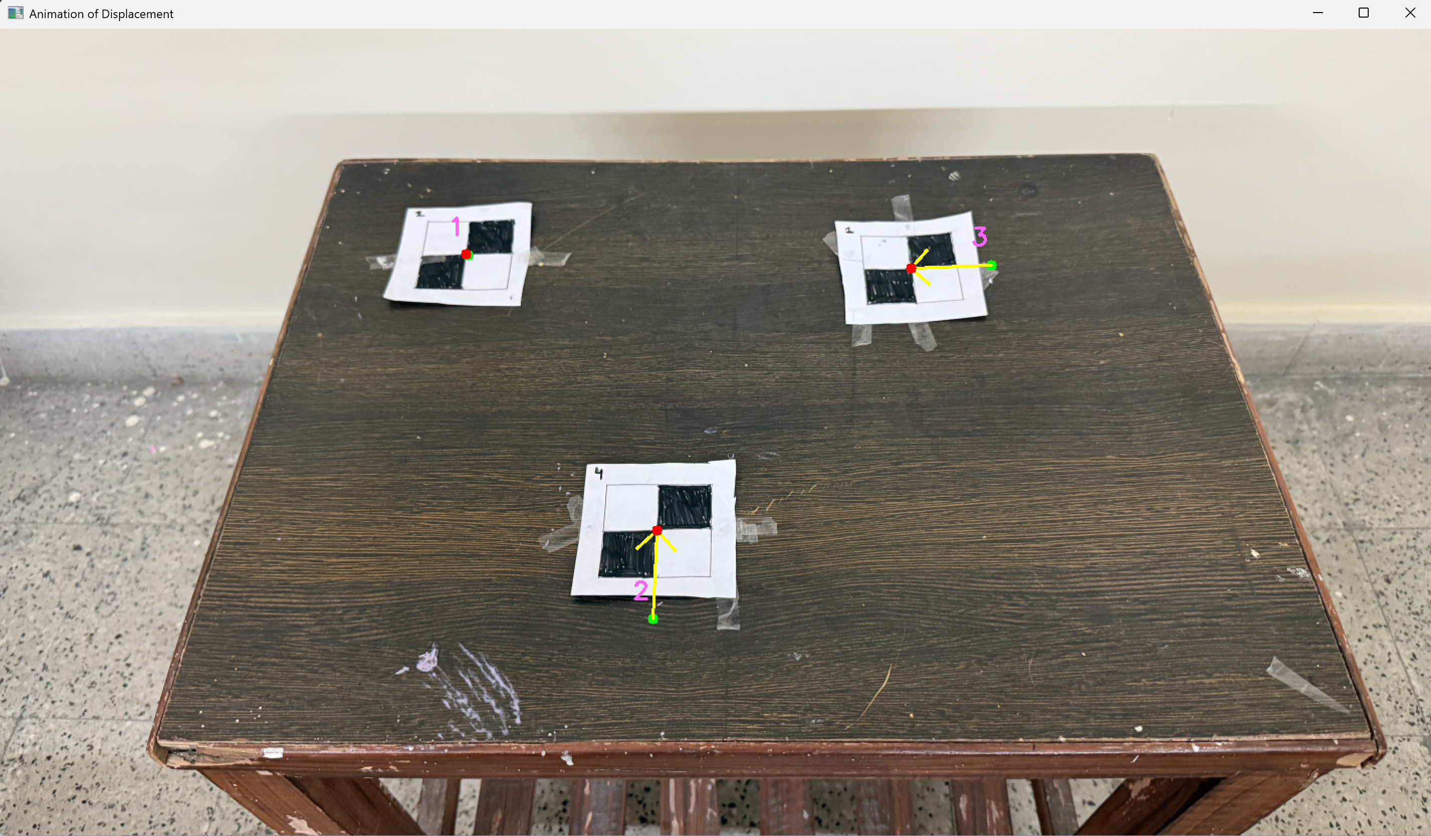
A 57.1 cm × 42.3 cm tabletop supplies a known dimension. With scale s = Lknown/Lpixels = 0.01703 units/pixel, each track becomes D = s√(Δx²+Δy²). The three reported tests compare 0.12 vs 0, 6.00 vs 5.5 and 5.45 vs 5.0, giving RMSE 0.394.

KLT displacement vectors on tabletop features
Detected corners, tracked endpoints and displacement vectors for the planar measurement test.
02 · ROAD-PLANE HOMOGRAPHY

Image motion becomes velocity

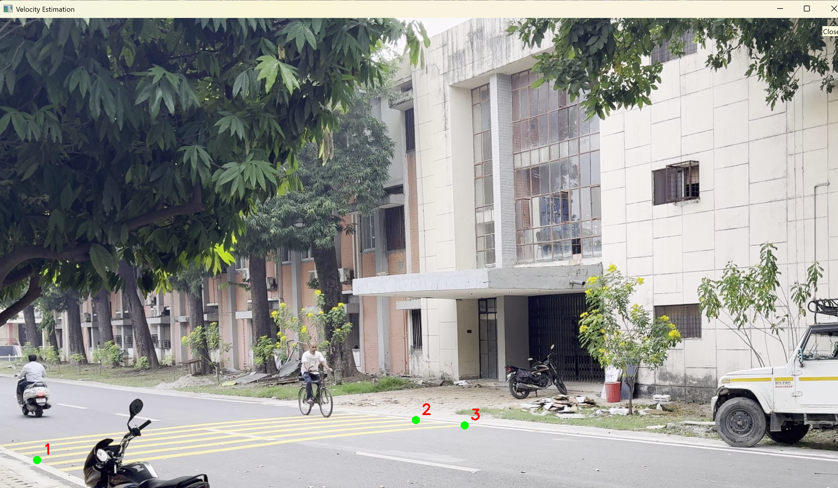
Four non-collinear road points estimate a projective transform x′ ~ Hx. Metric displacement is d = ‖X′t+1−X′t‖; velocity is v = d/Δt and converts to km/h by multiplying by 3.6.

Failure mode: the final spike occurs when a vehicle nears or exits the image boundary. Short/unstable tracks create a position jump, and differentiation amplifies it. Robust track rejection and temporal smoothing are the next controls.

03 · GLACIER CAMERA POSE

2D tracks are lifted into 3D context

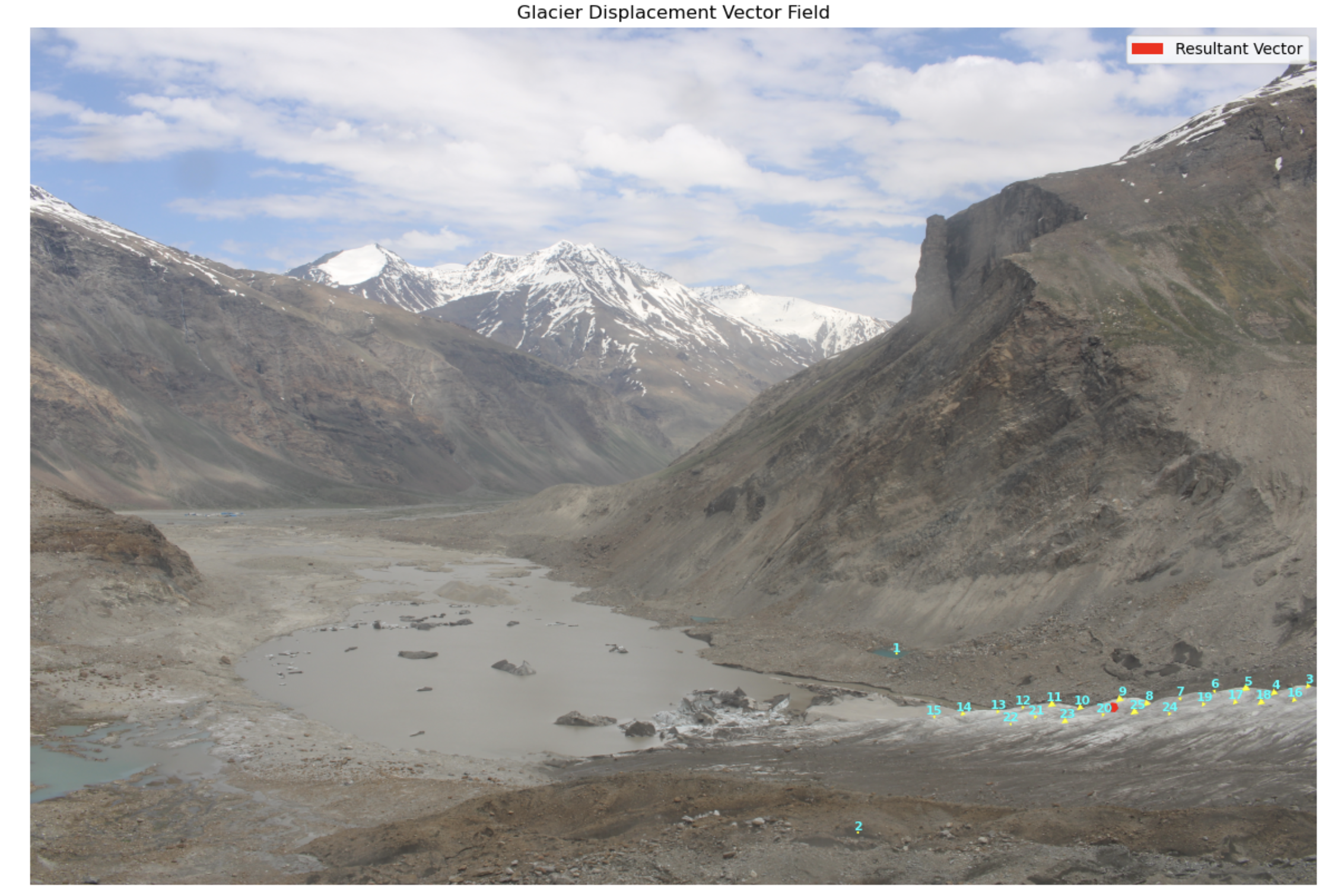
Ground-control correspondences solve s[x y 1]ᵀ = K[R|t][X Y Z 1]ᵀ with PnP. Pixel tracks are related to the calibrated scene geometry; the report uses an average ground-plane height of 4,120.68 m and GSD ≈ 0.273 m/pixel.

The mean optical-flow magnitude was 4.36 px, while the reported resultant 3D displacement was 25.24 m. Their non-linear relationship shows why a single global pixel-to-metre multiplier is unsafe under perspective.

Tracked glacier features and displacement vectors
Glacier feature tracks visualised as displacement vectors; pose and GCP quality dominate metric reliability.

What I would validate next

TRACK QUALITY

Forward–backward error

Reject drift where reverse tracking does not recover the original feature.

GEOMETRY

Reprojection residuals

Report GCP/image residuals and propagate calibration uncertainty into distance.

TEMPORAL

Robust motion model

Use median/RANSAC consensus and confidence-banded smoothing before differentiation.

TECHNICAL ASSIGNMENT

Satellite-image anomaly screening

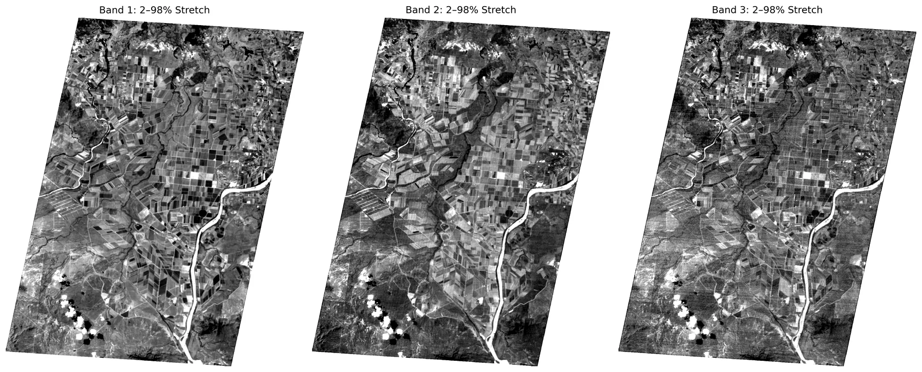
A reproducible workflow for three co-registered GeoTIFF bands that distinguishes screening evidence from confirmed sensor defects.

1523×1784 each band
26.23% NoData footprint
0.85–0.90 band correlation

Method and reasoning

01 · Metadata + NoData

Verify CRS, transform, bounds, type and alignment first. All bands share EPSG:4326 and grid geometry; the rotated blank border is not noise.

02 · Stretch + histograms

A 2–98% stretch reveals detail; histograms expose tails and repeated values without proving corruption.

03 · Median residual

R=I−median3×3(I) highlights local bright/dark deviations, but also roads and edges.

04 · Robust MAD

Zr=0.6745(R−median(R))/MAD. |Zr|>5 is a conservative, tunable screen that limits false positives.

05 · Profiles + cross-band evidence

Row/column profiles screen stripes; a single-band candidate is more suspicious than a feature present in all bands.

R(x)=I(x)−median3×3(I)(x)

The local residual removes slowly varying scene brightness. Large residual magnitude marks a pixel unlike its immediate neighbourhood—but edges can also respond.

Zr(x)=0.6745·(R(x)−median(R))/MAD(R)

The median absolute deviation is robust to heavy tails. A common screen of |Zr|>5 produces review candidates, not a defect verdict.

ρij=cov(Bi,Bj)/(σiσj)

Correlations of 0.850, 0.901 and 0.879 establish strong shared scene structure. A candidate unique to one band therefore deserves closer sensor-level review.

Band Candidate rate Interpretation
1 7.423% Highest response; includes edges.
2 2.358% Moderate response.
3 0.728% Lowest under same threshold.

Conclusion: grid geometry passes the consistency check, while 7.423%, 2.358% and 0.728% remain candidate rates only. A final defect label requires band identities, valid-range and saturation rules, sensor calibration information or trusted reference imagery. Cloud masking is intentionally not claimed because the Red/Green/NIR mapping was unknown.

ADDITIONAL WORK · DECISION SCIENCE · POINT CLOUDS

More geospatial projects

These projects show two complementary skills: multi-criteria spatial decision modelling and local-density reasoning over 3D point clouds.

FOREST FIRE · MULTI-CRITERIA DECISION ANALYSIS

Risk zonation with AHP and weighted overlay

Eight criteria—population density, LULC, elevation, slope, aspect, temperature, rainfall and wind speed—are converted to comparable risk scores. Pairwise AHP comparisons encode relative importance; the normalized priority vector becomes the parameter weight used in GIS overlay.

R(x) = Σi=1 8 wi·si(x)

si(x) is the reclassified susceptibility of criterion i at location x and Σwi=1. Consistency is checked with CI=(λmax−n)/(n−1) and CR=CI/RI≤0.10.

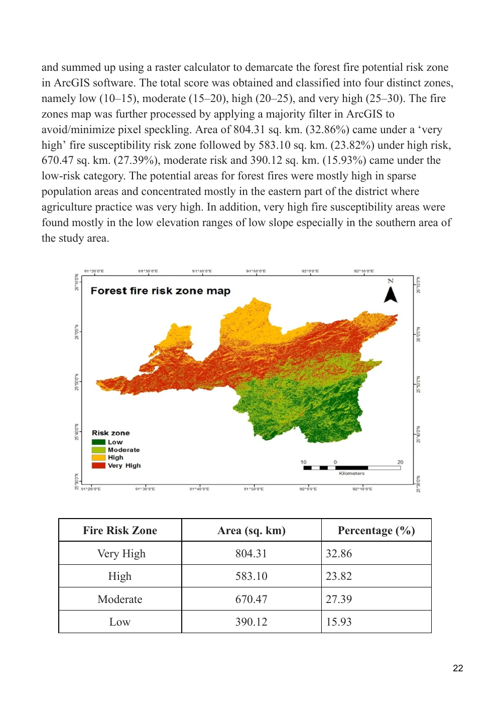
32.86% very-high risk 23.82% high risk 8 criteria

Validation logic: VIIRS/MODIS fire detections are overlaid on the ranked zones. A useful model should concentrate a larger share of observed detections in higher-risk classes; the map is susceptibility, not a real-time ignition forecast.

Forest fire risk zone map for Clarence Valley with area statistics
Clarence Valley risk classes produced by AHP-weighted raster overlay.
ONGOING · LIDAR QUALITY CONTROL

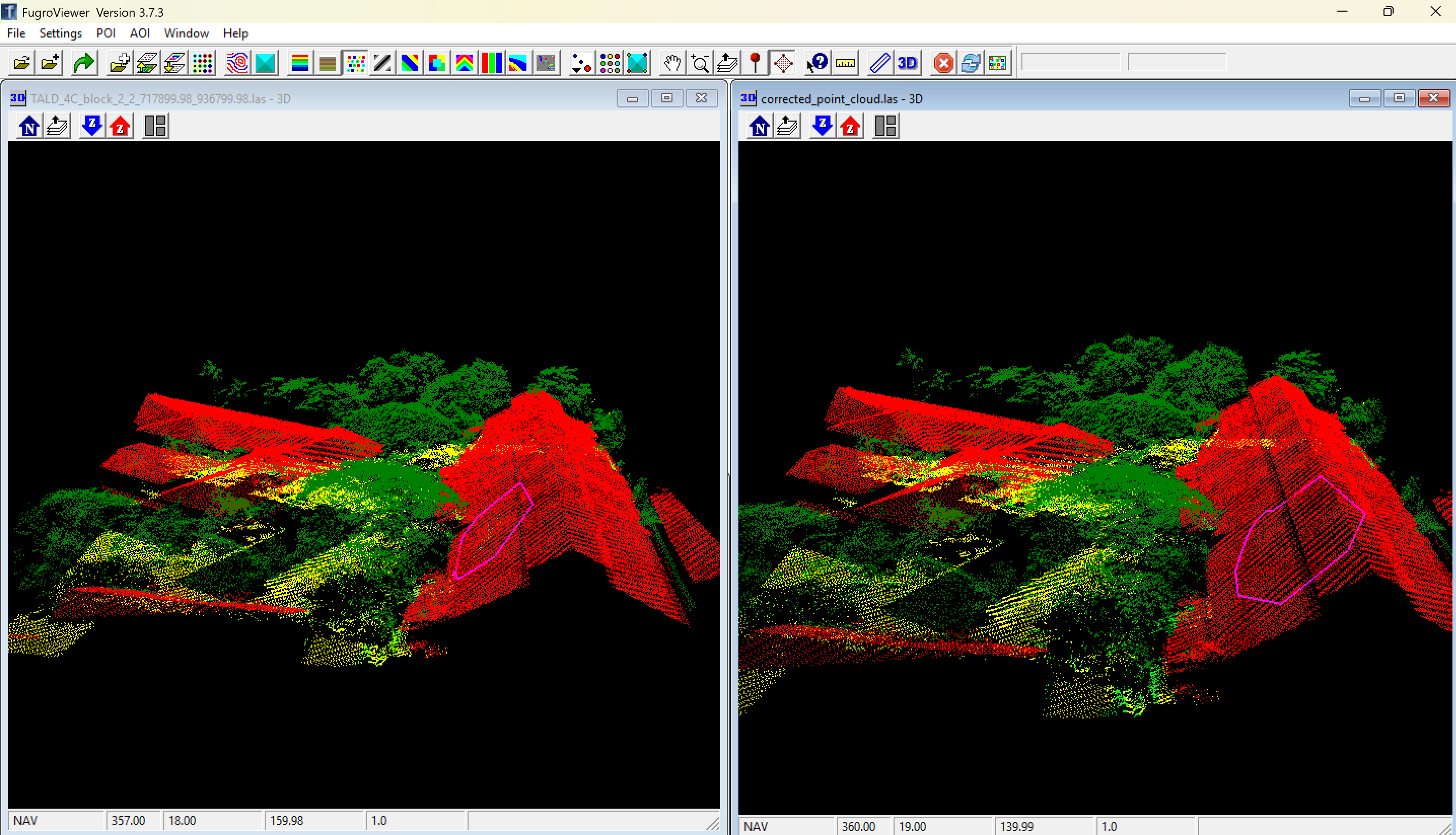
LiDAR point-cloud misclassification

The TALD block contains 182,600 points labelled as ground, shrubs, trees and buildings. Height above ground is estimated using nearest ground returns; three detectors are combined with logical OR: LOF, DBSCAN noise and class-specific height rules.

LOFk(p)=meano∈Nk(p) lrdk(o) / lrdk(p)

Local reachability density lrd compares p with nearby points, so LOF adapts to varying point density. The experiment uses k=70 and 0.5% contamination; DBSCAN uses ε=2.5 and minPts=15.

182,600 points 864 flagged 0.47% flagged share

Height rules flag shrubs above 25 m and trees above 36 m. Removal creates holes, so interpolation or completion is still proposed; PointNet++/RandLA-Net reclassification and F1/IoU evaluation remain future work. No post-correction accuracy gain is claimed.

Three-dimensional LiDAR point cloud classification view
3D point-cloud inspection used to reason about sparse local outliers and class inconsistencies.
ENVIRONMENTAL FORECASTING · NSUT

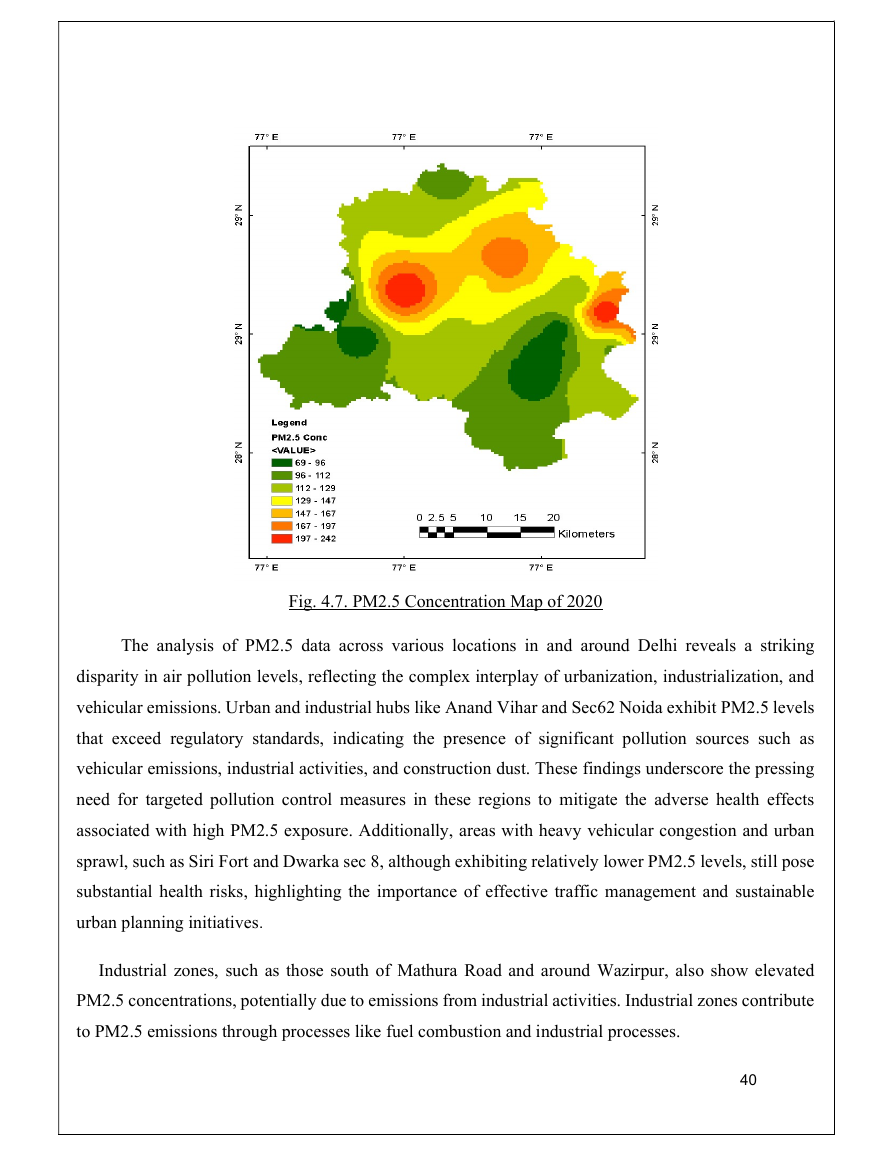
Delhi air-quality monitoring and prediction

PM2.5, PM10 and NO₂ surfaces, temporal trends and regression models connect spatial hotspots with forecast behaviour. Random Forest reported test R²=0.89, compared with 0.86 for linear regression.

R² = 1 − Σ(y−ŷ)² / Σ(y−ȳ)²

R² measures explained variation, not causal validity. Time-aware splitting, residual diagnostics and uncertainty bands are required before operational use.

2015–20 analysis period 0.88 PM2.5–AQI correlation 0.89 RF test R²

IIST · PRACTICAL LABS & MINI PROJECTS

Coursework that connects equations to evidence.

These are working implementations—not a list of subjects. Each study begins with a measurable problem, applies a reproducible algorithm and ends with a visual output that can be audited.

COMPUTER VISION · LAB 02

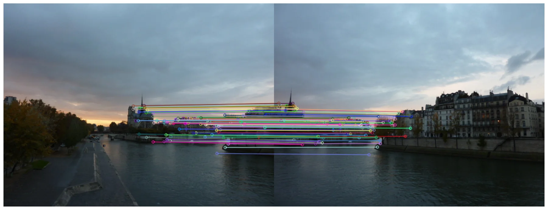
Image stitching through feature geometry

Two overlapping Paris photographs are converted into one panorama. SIFT detects scale- and rotation-tolerant keypoints, brute-force matching compares descriptors, and RANSAC rejects correspondences that do not support one consistent projective transformation.

DetectSIFT keypoints
→
MatchL2 descriptor distance
→
EstimateRANSAC homography
→
Warpcompose panorama
x′ ∼ Hx ··· I={i: ‖x′ᵢ−π(Hxᵢ)‖₂<τ}

H is a 3×3 homography with eight independent degrees of freedom. At least four non-collinear pairs are required; RANSAC keeps the largest reprojection-consistent inlier set.

204 brute-force matches145 good KNN matches3×3 homography
GIS MINI PROJECT · FIELD DATA ENGINEERING

Spatial tree database for the IIST campus

Field observations become a queryable GIS layer: record coordinates, height and perimeter at breast height; attach taxonomy and use attributes; validate the table; then map distribution and inspect each tree spatially.

DBH ≈ PBH / π

Circumference measured at 1.3 m is converted to diameter; the cleaned table agrees within a mean absolute difference of about 0.27 cm.

G = π(DBH/2)²

Basal area turns diameter into a comparable structural measure for each stem.

H′ = −Σ pᵢ ln(pᵢ)

Shannon diversity uses each species share pᵢ; the cleaned records yield H′=3.347.

197 usable records51 common-name groups6.67 m mean height

Data-QA finding: the presentation reports 202 readings and 58 varieties, while the supplied cleaned CSV contains 197 rows and 51 populated common-name categories. Site metrics use the auditable table and preserve the discrepancy instead of silently mixing versions.

MICROWAVE REMOTE SENSING · GOOGLE EARTH ENGINE

Crop classification: Sentinel-1 versus Sentinel-2

For Ranijot village, the same six-class sampling design and 70/30 split compare radar and optical evidence. Sentinel-1 uses VV/VH after a 50 m focal-median speckle filter; Sentinel-2 uses ten reflectance bands plus NDVI after QA60 cloud masking. Each branch feeds a 50-tree Random Forest.

Sample6 classes × 25
→
PrepareSAR / optical
→
EngineerVV,VH / bands,NDVI
→
TrainRF · 50 trees
→
ValidateOA + κ
NDVI=(B8−B4)/(B8+B4)

Near-infrared and red contrast provides a vegetation-vigour feature.

ŷ(x)=mode{hₜ(x)}ₜ₌₁⁵⁰

Random Forest predicts by majority vote across 50 decision trees.

κ=(pₒ−pₑ)/(1−pₑ)

Kappa adjusts observed agreement for agreement expected by chance.

SENTINEL-1 SAR62.29%κ = 0.475
SENTINEL-2 OPTICAL90.16%κ = 0.866

Interpretation: optical features generalised better in this experiment. The SAR median composite suppresses temporal crop phenology; multi-date VV/VH trajectories, textures and radar vegetation indices are the logical next tests. Anonymised Crop A–E labels also limit agronomic interpretation.

SELECTED COMPUTER-VISION LABS

Three methods, three kinds of structure

POINT STRUCTURE

Harris corners

M=Σw[[Iₓ²,IₓIᵧ],[IₓIᵧ,Iᵧ²]]R=det(M)−k·trace(M)²

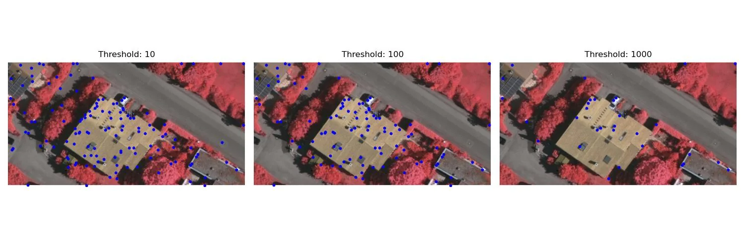
Large positive R means intensity changes strongly in two directions. Raising the response threshold reduced detections from 130 to 100 to 31—an explicit repeatability-versus-selectivity trade-off.

LINE STRUCTURE

Hough deskew

ρ=x cosθ+y sinθ

Edge pixels vote in (ρ,θ) space; the dominant peak estimates document orientation. Otsu thresholds of 0.365 and 0.338 supported detected skews of −16° and −13°, which were corrected by rotation.

APPEARANCE STRUCTURE

Bag of visual words

w(f)=arg minₖ ‖f−μₖ‖²hₖ=nₖ/Σⱼnⱼ

SIFT descriptors are quantised into 100 K-means words. Normalised image histograms feed 5-NN across 101 Caltech classes; the recorded 80/20 experiment reached 37.85% accuracy.

VERIFIED LEARNING & RECOGNITION

Credentials aligned with the work.

Selected achievements and courses reinforce the same themes visible in the projects: remote sensing, spatial analysis, machine learning, cloud systems and quantitative research.

Recognition

2025

WorldQuant PowerPool Alpha Competition

94th global rank

Competitive quantitative-research result built on simulation, risk and robustness checks.

2023

WorldQuant Brain NSUT Alphathon

6th place

Recognised for outstanding performance in the NSUT Alphathon.

2025

GATE

AIR 153

National-level performance supporting advanced geospatial engineering study.

2014 · GOVERNMENT OF MAHARASHTRA

Intermediate Grade Drawing Examination

Qualified with B grade

State-level assessment across observational drawing, memory/object drawing, design, geometry and lettering; the result contributed 10 grace marks to the SSC total.

Selected certifications

NPTEL · IIT Kharagpur Cloud Computing · Jan–Apr 2024 · 12 weeks · Elite · 80% Official NPTEL certificate ↗
IIRS–ISRO Machine Learning to Deep Learning: A Journey for Remote Sensing Data Classification · 4–8 Jul 2022 · 13 h 30 m
IIRS–ISRO Geo-spatial Applications for Forest Ecosystem Analysis · 20–25 Jun 2022 · 7 h 30 m
Esri Going Places with Spatial Analysis · 6 weeks · completed 23 Mar 2023
Udemy Machine Learning & Deep Learning in Python & R · 33 hours · completed 28 Jun 2023
IIST + National Centre for Geodesy, IIT Kanpur Precision Mapping: Geodesy, DGPS, and Drones for Surveying and Mapping · 22–24 Oct 2024

Privacy: credentials are summarized from verified records without publishing private storage links or document identifiers.

PROFESSIONAL · PROJECT EVIDENCE

Internships explained through the systems I built.

Each engagement is presented as a problem → method → output chain, with the real report figures that best explain the work.

HIWARA ENGINEERS · GEOSPATIAL INTERN · 2026

Antariksh-JEPA retrieval system

I developed and evaluated a bidirectional optical↔SAR retrieval pipeline: paired BigEarthNet-MM tiles enter dual Vision Transformers, JEPA-style latent prediction and contrastive alignment bring modalities together, and 192-bit hashes support fast Hamming search.

dH(bq,bi) = popcount(bq XOR bi)

Lower Hamming distance means more matching bits. Retrieval quality is evaluated with average precision over the ranked top-k list, then averaged over queries.

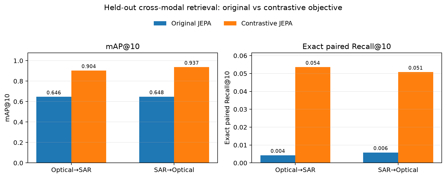
0.9036 optical→SAR mAP@10 0.9369 SAR→optical mAP@10 24 bytes per code
Open full Antariksh case study →
Original and contrastive cross-modal retrieval comparison
Cross-modal retrieval comparison used to inspect how contrastive alignment changes ranked results.
CRIS · SOFTWARE INTERN · JUN–SEP 2023

Railway inspection and marketing workflows

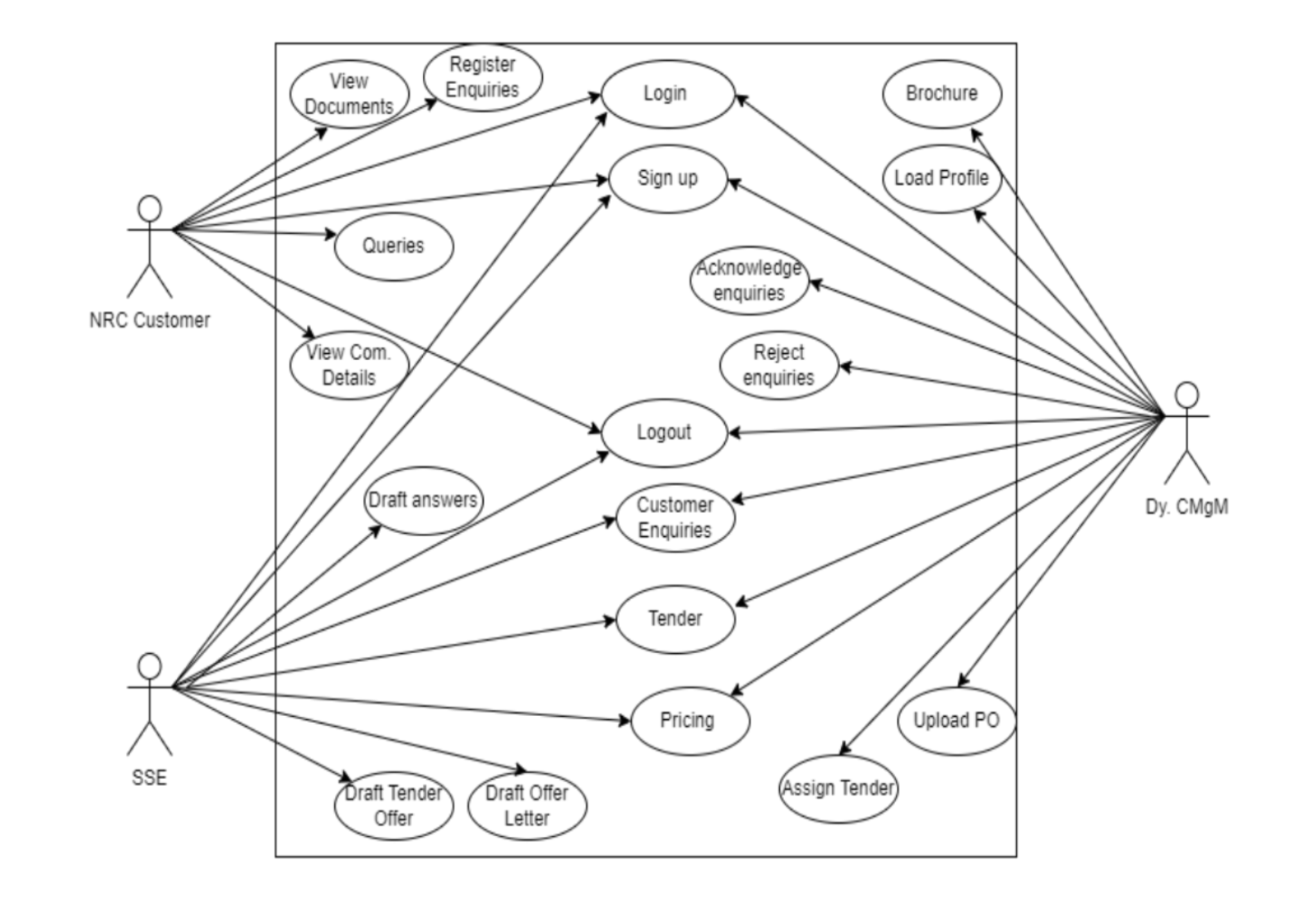
I translated roles and requirements into Django/PostgreSQL workflows for BLW: inspection-sheet CRUD, validation, session controls and forms for locomotive, DG-set and spare-parts processes. A JavaScript countdown exposed remaining session time and offered extension before automatic logout.

User action → validation → Django view → PostgreSQL → role-filtered response

The DFD separates NRC customers, SSE staff and the nodal officer. Role-based transitions prevent every actor from editing every state, while validation rules protect data integrity.

19 numbered tasks 16 marked completed 3 not allotted

Engineering boundary: the report documents implementation and deployment on a railway trial server; it does not provide an independent production-security audit.

NIDM · GIS INTERN · 2023

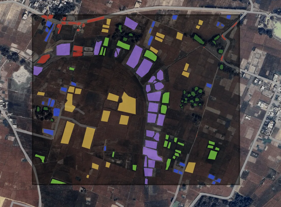
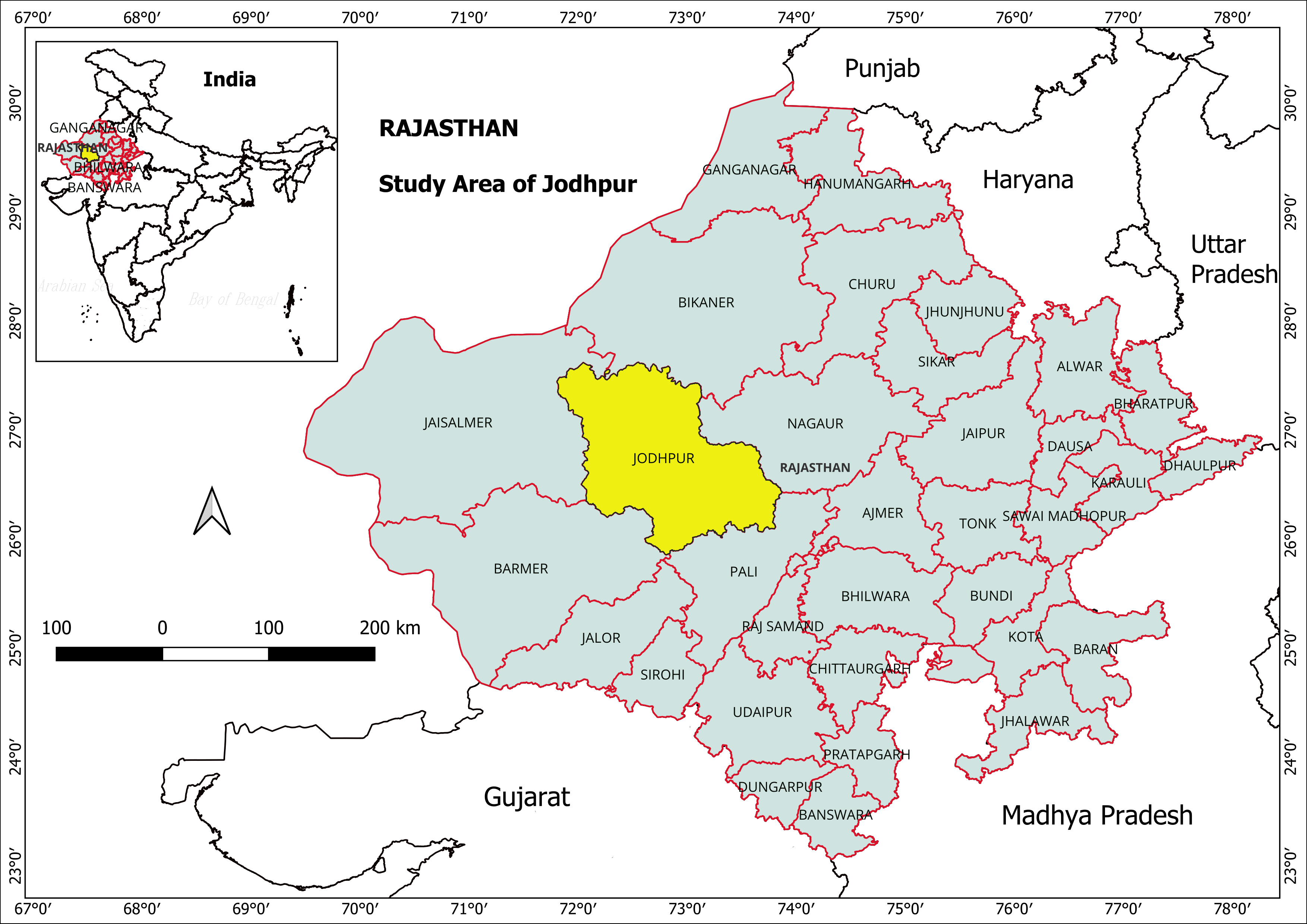
Jodhpur heritage and disaster-exposure mapping

I cleaned administrative boundaries, geocoded heritage locations and integrated satellite context into analysis-ready layers. The logic is spatial: normalize coordinates and CRS, join each asset to its administrative unit, compute proximity/exposure relationships, then design cartography for report use.

d(p,H) = minh∈H distance(p,h)

For each heritage asset p, proximity to a hazard feature set H can be used as an exposure indicator. Distances are meaningful only after choosing an appropriate projected CRS.

Jodhpur district context GIS layer integration Maps decision output

Continuing research experience

Brain Research Consultant · WorldQuant

Alpha research through hypothesis design, simulation, turnover/risk inspection and robustness refinement; the role is documented separately from academic internships.

Toolkit

ML

Python · PyTorch · OpenCV · scikit-learn

Spatial

Rasterio · GeoPandas · PostGIS · GEE

Remote sensing

Optical · SAR · LiDAR · Photogrammetry

Product

Django · PostgreSQL · Streamlit · Git

POSITIONS OF RESPONSIBILITY · VERIFIED RECORDS

Leadership as coordination, service and accountable delivery.

The roles below are not presented as titles alone—the diagram shows who depended on the role, what responsibility was carried and what evidence supports it.

Placement coordination across two institutes

CURRENT · SEP 2025–PRESENT

Placement Coordinator · IIT Roorkee

Placement & Internship Cell

  • Targeted recruiter and HR outreach aligned to student profiles and organisational needs.
  • Coordinates Job Announcement Forms and Summer Internship Forms so requirements, eligibility and timelines stay explicit.
  • Supports on-campus logistics, candidate communication, assessments and interview flow.
← progression
SEP 2024–JUN 2025

Placement Coordinator · IIST

Department of Geoinformatics

  • Connected student profiles, departmental coordination and recruiter communication.
  • Maintained schedule continuity and supported candidate/interview logistics.
  • Tenure formally confirmed by the Head, Centre for Career Guidance and Placements.

Current role: stakeholder operating model

SEP 2025–PRESENT Placement Coordinator Placement & Internship Cell · IIT Roorkee
↙
Students collect profiles · communicate opportunities · coordinate schedules
↓
Career office & faculty JAF/SIF workflow · eligibility · calendar · process continuity
↘
Recruiters targeted outreach · requirement clarity · assessment and interview logistics

Operating logic: recruiter requirements become a structured opportunity; eligible candidates receive one clear timeline; assessments and interviews are coordinated; completion status and feedback close the process loop.

National Service Scheme

2022–2024

NSS Volunteer · NSUT West Campus

240 service hours

Completed the documented service requirement and a seven-day special camp; the official volunteer register also lists the role for 2022–23.

23–29 MAY 2022

National Integration Camp

7-day residential camp

Participated in the Ministry of Youth Affairs & Sports / Regional Directorate of NSS camp hosted at NSUT, working in a multi-institution service setting.

OPERATING LOGIC

Plan → mobilise → deliver → document

service workflow

Volunteer work converts coordination into observable delivery: assign responsibilities, execute activities, record participation and close the loop with evidence.

Responsibility principles

TRACEABILITY

Make ownership visible

Every task needs an owner, a deadline and a verifiable completion state.

COMMUNICATION

Reduce hand-off loss

Translate requirements between students, faculty, officials and external stakeholders.

SERVICE

Measure delivery

Hours, participation and completed activities make contribution auditable.

Press Ctrl K to open search.